Reference¶

Layers¶

Linear Regression¶

class theano_wrapper.layers.LinearRegression(regularizer_fn=None, shape=None, X=None)¶

Simple Linear Regression. Linear regression is a linear predictor modeling the relationship between a scalar dependent variable $y$ and one or more explanatory variables denoted $D$ from an input sample $X$ . The target value is given by the formula:

$y = \sum_{i=0}^{|\mathcal{D}|} (W_i \cdot X_i) + b$

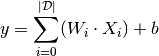
Parameters:	n_in (int) – Number of input nodes n_out (int) – Number of output nodes

X¶: theano variable – Symbolic input.

y¶: theano variable – Symbolic output.

W¶: theano variable – Weights matrix, shape=(n_in, n_out).

b¶: theano variable – Bias vector, shape=(n_out,).

predict¶: theano expression – Predict target value for input X.

cost¶: theano expression – Mean squared error loss function.

Logistic Regression¶

class theano_wrapper.layers.LogisticRegression(regularizer_fn=None, shape=None, X=None)¶

Multi-class Logistic Regression.

Logistic regression is a probabilistic, linear classifier. It is parametrized by a weight matrix $W$ and a bias vector $b$ . Classification is done by projecting an input vector onto a set of hyperplanes, each of which corresponds to a class. The distance from the input to a hyperplane reflects the probability that the input is a member of the corresponding class.

$P(Y=i|x, W,b) &= softmax_i(W x + b) \\ &= \frac {e^{W_i x + b_i}} {\sum_j e^{W_j x + b_j}}$

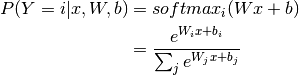
The model’s prediction $y_{pred}$ is the class whose probability is maximal, specifically:

$y_{pred} = {\rm argmax}_i P(Y=i|x,W,b)$

Parameters:	n_in (int) – Number of input nodes n_out (int) – Number of output nodes

X¶: theano variable – Symbolic input.

y¶: theano variable – Symbolic output.

W¶: theano variable – Weights matrix, shape=(n_in, n_out).

b¶: theano variable – Bias vector, shape=(n_out,).

predict¶: theano expression – Return the most probable class (the probability function as described above).

cost¶: theano expression – Negative log-likelihood if we define the likelihood $\cal{L}$ and loss $\ell$ :

$\mathcal{L} (\theta=\{W,b\}, \mathcal{D}) = \sum_{i=0}^{|\mathcal{D}|} \log(P(Y=y^{(i)}|x^{(i)}, W,b)) \\ \ell (\theta=\{W,b\}, \mathcal{D}) = - \mathcal{L} (\theta=\{W,b\}, \mathcal{D})$

probas¶: theano expression – Calculate probabilities for input X.

Multi-layer Regression¶

class theano_wrapper.layers.MultiLayerRegression(n_in, n_hidden, n_out, random=None)¶

Multilayer Regression.

An MLP can be viewed as a linear regression predictor where the input is first transformed using a transformation $\Phi$ . This transformation projects the input data into a more sparse or dense space. This intermediate layer is referred to as a hidden layer. Formally, a one-hidden-layer MLP is a function $f: R^D \rightarrow R^L$ , where $D$ is the size of input vector $x$ and $L$ is the size of the output vector $f(x)$ , such that, in matrix notation: .. math:

f(x) = G( b^{(2)} + W^{(2)}( s( b^{(1)} + W^{(1)} x))),

with bias vectors $b^{(1)}$ , $b^{(2)}$ ; weight matrices $W^{(1)}$ , $W^{(2)}$ and activation functions $G$ and $s$ . The vector $h(x) = \Phi(x) = s(b^{(1)} + W^{(1)} x)$ constitutes the hidden layer. $W^{(1)} \in R^{D \times D_h}$ is the weight matrix connecting the input vector to the hidden layer. Each column $W^{(1)}_{\cdot i}$ represents the weights from the import input units to the i-th hidden unit. This estimator’s $s$ is the Rectified linear unit output, or $relu$ function.

Parameters:

n_in (int) – number of input nodes
n_hidden (int or list(int)) – if int this is the number of hidden layer nodes in a single-hidden-layer network. If list of int’s this is a list of number of nodes for len(n_hidden) successive layers
n_out (int) – number of output nodes
random (Optional(int or numpy.random.RandomState instance)) – an integer seed or random state generator. Default: None, links to np.random

layers¶: list – List of all the estimator layers with layers[0] being the input layer, layer[1:-1] being the hidden layers and layers[-1] the output layer.

X¶: theano variable – Symbolic input of first layer.

y¶: theano variable – Symbolic output of last layer.

params¶: list – Vector of all the estimator parameters, i.e. weights and biases of all the layers

predict¶: theano expression – Return the most probable class (the probability function as described above).

cost¶: theano expression – Negative log-likelihood from LogisticRegression.

Multi-Layer Perceptron¶

class theano_wrapper.layers.MultiLayerPerceptron(n_in, n_hidden, n_out, random=None)¶

Multilayer Perceptron.

An MLR can be viewed as a logistic regression classifier where the input is first transformed using a learnt non-linear transformation $\Phi$ . This transformation projects the input data into a space where it becomes linearly separable. This intermediate layer is referred to as a hidden layer.

Formally, a one-hidden-layer MLR is a function $f: R^D \rightarrow R^L$ , where $D$ is the size of input vector $x$ and $L$ is the size of the output vector $f(x)$ , such that, in matrix notation:

$f(x) = G( b^{(2)} + W^{(2)}( s( b^{(1)} + W^{(1)} x))),$

with bias vectors $b^{(1)}$ , $b^{(2)}$ ; weight matrices $W^{(1)}$ , $W^{(2)}$ and activation functions $G$ and $s$ . The vector $h(x) = \Phi(x) = s(b^{(1)} + W^{(1)} x)$ constitutes the hidden layer. $W^{(1)} \in R^{D \times D_h}$ is the weight matrix connecting the input vector to the hidden layer. Each column $W^{(1)}_{\cdot i}$ represents the weights from the import input units to the i-th hidden unit. This estimator’s $s$ is the $tanh$ function.

Parameters:

n_in (int) – number of input nodes
n_hidden (int or list(int)) – if int this is the number of hidden layer nodes in a single-hidden-layer network. If list of int’s this is a list of number of nodes for len(n_hidden) successive layers
n_out (int) – number of output nodes
random (Optional(int or numpy.random.RandomState instance)) – an integer seed or random state generator. Default: None, links to np.random

layers¶: list – List of all the estimator layers with layers[0] being the input layer, layer[1:-1] being the hidden layers and layers[-1] the output layer.

X¶: theano variable – Symbolic input of first layer.

y¶: theano variable – Symbolic output of last layer.

params¶: list – Vector of all the estimator parameters, i.e. weights and biases of all the layers

predict¶: theano expression – Return the most probable class (the probability function as described above).

cost¶: theano expression – Negative log-likelihood from LogisticRegression.

Trainers¶

Epoch-based¶

class theano_wrapper.trainers.EpochTrainer(clf, alpha=0.01, max_iter=10000, patience=5000, p_inc=2.0, imp_thresh=0.995, random=None, verbose=None)¶

Simple epoch-based trainer using Gradient Descent with patience. The idea is that we train for at least n (patience) epochs and then if the score keeps getting better (biased by imp_thresh) we elongate the training session by a factor of p_inc.

Parameters:

clf – the estimator to train
alpha (float) – learning rate
max_iter (int) – max_iterations to go through
patience (int) – look at least that many samples
p_inc (float) – how many more samples to fit after each improvement
imp_thresh (float) – the limit of what to consider improvement
random (int or random state generator) – a random state for predictable results
verbose (int) – verbosity factor. None = off, n = every n periods

gradients¶: theano symbolic function – The gradient for each parameter.

updates¶: theano symbolic function – Compute update values.

fit(X, y)¶: Train estimator using input samples. This implementation will automatically split the input into an 80% training and an 20% validation set

predict(X)¶: Return estimator prediction for input X

Stohastic Gradient Descent¶

class theano_wrapper.trainers.SGDTrainer(clf, batch_size=None, alpha=0.01, max_iter=10000, patience=5000, p_inc=2.0, imp_thresh=0.995, random=None, verbose=None)¶

Stohastic Gradient descent trainer with patience. This classifier works in a similar way to EpochTrainer, but instead of fitting all the samples it splits them to minibatches and go through a subset of all the samples at a fit period. This allows for speed improvements with large datasets and off-line training, i.e. training without all the samples available at once.

Parameters:

clf – the estimator to train
batch_size (int or None) – how many samples to consider for each training batch. if None, it is set to int(n_samples/100)
alpha (float) – learning rate
max_iter (int) – max_iterations to go through
patience (int) – look at least that many samples
p_inc (float) – how many more samples to fit after each improvement
imp_thresh (float) – the limit of what to consider improvement
random (int or random state generator) – a random state for predictable resi;ts
verbose (int) – verbosity factor. None = off, n = every n periods

gradients¶: (theano symbolic function) The gradient for each parameter

updates¶: (theano symbolic function) Compute update values

fit(X, y)¶: Train estimator using input samples. This implementation will automatically split the input into an 80% training and an 20% validation set

predict(X)¶: Return estimator prediction for input X

Regularizers¶

L1 / L2 squared¶

theano_wrapper.trainers.l1_l2_reg(l1_reg=0.0, l2_reg=0.0001)¶

L1 and L2 squared regularization.

L1 and L2 regularization involve adding an extra term to the loss function, which penalizes certain parameter configurations. For a loss function $\ell(\theta, \cal{D})$ of the prediction function f parameterized by $\theta$ on data set $\cal{D}$ , the regularized loss will be:

$E(\theta, \mathcal{D}) = \ell(\theta, \mathcal{D}) + \lambda R(\theta)\\$

or, in our case:

$E(\theta, \mathcal{D}) = NLL(\theta, \mathcal{D}) + \lambda||\theta||_p^p$

where

$||\theta||_p = \left(\sum_{j=0}^{|\theta|}{|\theta_j|^p}\right)^{\frac{1}{p}}$

$\theta$ is a set of all parameters for a given model, $\lambda$ the hyper-parameter which controls the relative importance of the regularization parameter and $R$ the regularization function. Commonly used values for $p$ are 1 and 2, hence the L1/L2 nomenclature. If $p=2$ , then the regularizer is also called “weight decay”.

In this model both L1 and L2 regularization is supported.

Parameters:

clf – an estimator
l1_reg (float) – The l1 regularization parameter. Defaults to .0
l2_reg (float) – The l2 regularization parameter. Defaults to .0001

Returns:

Symbolic expression that calculates the: regularized cost.

Return type:

cost (theano expression)

Example:

clf = SomeClassifier(*args)
reg = l1_l2_reg(clf, 0.0001, 0.001)
trn = SomeTrainer(clf, reg=reg)
[...]